
contentiousR creates reproducible country-year panels
for contentious politics and civil conflicts research, offers
diagnostics and visualization tools, and allows interoperation with
peacesciencer. Every public loader supports Correlates of
War ("cow") and Gleditsch-Ward ("gw") country
codes.
Build and enrich a panel
Construct a state panel, then add data.
library(contentiousR)

panel <- build_states_panel(
  start_year = 2000,
  end_year = 2002,
  coding_system = "cow"
)

analysis_data <- panel |>
  add_gdp() |>
  add_conflict("ucdp_prio") |>
  add_leader_data("archigos")

analysis_data[1:4, c(
  "country", "year", "gdp_pcap", "ucdp_prio_incidence", "leader"
)]
#>         country year gdp_pcap ucdp_prio_incidence    leader
#> 1 United States 2000 55889.52                  NA   Clinton
#> 2 United States 2001 55783.75                   1 G.W. Bush
#> 3 United States 2002 56127.44                   1 G.W. Bush
#> 4        Canada 2000 48531.95                  NA  Chretien
An unmatched row remains NA, as a source may not cover a
country-year.
Load data separately
Standalone loaders are useful when you want to inspect or aggregate data before joining them.
conflicts <- conflict_data(
  start_year = 2000,
  end_year = 2002,
  dataset = "ucdp_prio",
  coding_system = "gw"
)

head(conflicts)
#> # A tibble: 6 × 13
#>      gw  year ucdp_prio_incidence ucdp_prio_onset ucdp_prio_n_conflicts
#>   <int> <dbl>               <int>           <int>                 <int>
#> 1     2  2001                   1               1                     2
#> 2     2  2002                   1               0                     1
#> 3   100  2000                   1               0                     1
#> 4   100  2001                   1               0                     1
#> 5   100  2002                   1               0                     1
#> 6   200  2001                   1               1                     1
#> # ℹ 8 more variables: ucdp_prio_intensity_max <int>, ucdp_prio_war <int>,
#> #   ucdp_prio_cumulative_intensity <int>, ucdp_prio_type_max <int>,
#> #   ucdp_prio_intrastate <int>, ucdp_prio_interstate <int>,
#> #   ucdp_prio_incompatibility_max <int>, ucdp_prio_ep_end <int>
UCDP/PRIO distinguishes active conflict-years
(ucdp_prio_incidence) from the first year of an episode
(ucdp_prio_onset). See
vignette("data-sources", package = "contentiousR") before
interpreting any source-specific variable.
Conflict spells (peace-years)
add_spell_duration() turns a binary conflict column into
a duration counter — years since the last event for that state,
restarting after each new one. This is the same construct as
peacesciencer::add_spells() (named differently here to
avoid colliding with it when both packages are attached), useful as a
control for temporal dependence in event-history models (e.g. with cubic
splines). It needs a column without NA, so filter
first:
spell_data <- build_states_panel(1990, 2005, coding_system = "gw") |>
  add_conflict("ucdp_prio") |>
  tidyr::drop_na(ucdp_prio_onset) |>
  add_spell_duration(event = "ucdp_prio_onset")

spell_data[spell_data$gw == 2, c("gw", "year", "ucdp_prio_onset", "ucdp_prio_spell")]
#>   gw year ucdp_prio_onset ucdp_prio_spell
#> 1  2 2001               1               0
#> 2  2 2002               0               0
#> 3  2 2003               1               1
#> 4  2 2004               0               0
#> 5  2 2005               0               1
If event is omitted, add_spell_duration()
looks for exactly one column ending in _onset,
_incidence, or _ongoing and uses that; it
errors if none or several are found. _onset-style columns
treat every 1 as an independent event by default;
_incidence/_ongoing-style columns collapse a
run of consecutive 1s into one event, leaving the
continuation years NA in the output (override this with the
ongoing argument).
Lagged variables
add_lag() adds a lagged version of one or more columns,
computed within each state after sorting by year and grouping by state
before lagging. Unlike a plain dplyr::lag(), it checks that
the preceding row is genuinely n years earlier, so a gap in
the year sequence produces NA rather than silently reaching
further back than intended:
build_states_panel(1990, 1995, coding_system = "cow") |>
  add_gdp() |>
  add_lag(vars = c("gdp_pcap", "gdp_growth"), n = 1) |>
  dplyr::filter(cow == 2) |>
  dplyr::select(cow, year, gdp_pcap, gdp_pcap_l, gdp_growth_l)
#> # A tibble: 6 × 5
#>     cow  year gdp_pcap gdp_pcap_l gdp_growth_l
#>   <dbl> <dbl>    <dbl>      <dbl>        <dbl>
#> 1     2  1990   45755.        NA         NA
#> 2     2  1991   45035.     45755.         3.18
#> 3     2  1992   45912.     45035.        -1.58
#> 4     2  1993   46485.     45912.         1.95
#> 5     2  1994   47696.     46485.         1.25
#> 6     2  1995   48326.     47696.         2.60
Each requested variable gets one new column named
<var>_l. Call add_lag() again
(optionally with a different n) for additional lags.
Visualizing onsets
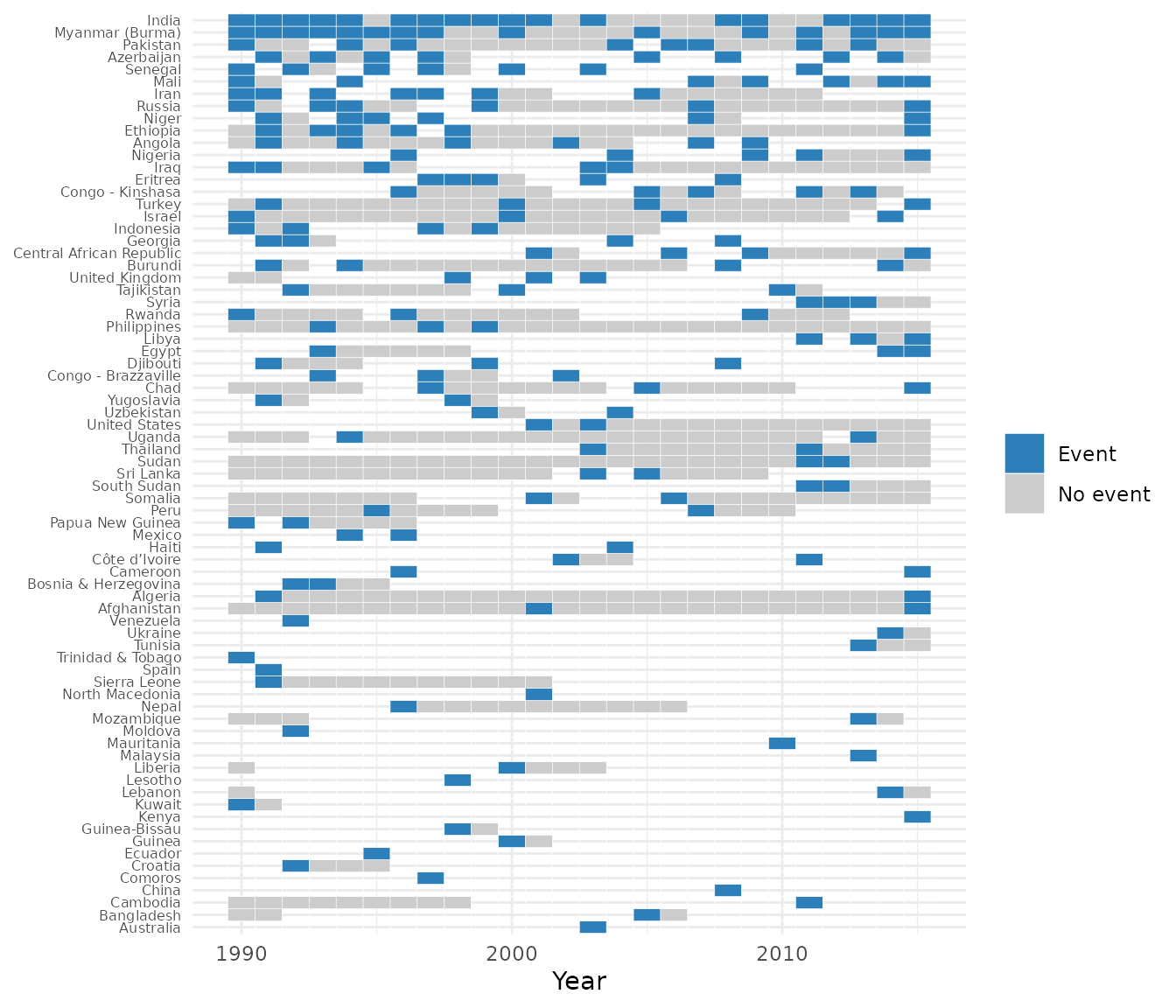
plot_coverage() draws a state-by-year heatmap of a
binary (0/1) event column: 1 years are shaded as an event,
0 years as no event, and years where the source has no data
— either var is NA, or the state does not
appear in the panel that year at all, e.g. before independence — are
left blank. States that never have the event are dropped by default
(drop_empty = TRUE), since an all-blank/grey row adds
clutter without showing where events actually happened.
if (requireNamespace("ggplot2", quietly = TRUE)) {
  build_states_panel(1990, 2015, coding_system = "cow") |>
    add_conflict("ucdp_prio") |>
    plot_coverage("ucdp_prio_onset")
}
Optional V-Dem data
V-Dem is not bundled and its R data package is not on CRAN. Install it from its official repository, then request only the indicators you need:
build_states_panel()
Creates a state-year panel with optional filters:
panel <- build_states_panel(
  start_year        = 1946,
  end_year          = 2019,
  coding_system     = "cow",   # or "gw"
  exclude_microstates = TRUE,
  exclude_non_un    = TRUE,
  exclude_islands   = FALSE
)
load_gdp_data() / add_gdp()
Two GDP sources are available via dataset.
"gapminder" (default) returns gdp_pcap,
log_gdp_pcap, and gdp_growth.
"fariss" returns the latent GDP and GDP per capita
estimates from Fariss, Anders, Markowitz, and Barnum (2022) as
fariss_gdp and fariss_gdppc, with much wider
coverage (1500–2019) but units that are not independently verified in
this package — see
vignette("data-sources", package = "contentiousR").
# Standalone
gdp <- load_gdp_data(start_year = 1990, end_year = 2015, coding_system = "cow")
fariss_gdp <- load_gdp_data(1700, 2015, dataset = "fariss", coding_system = "cow")

# Pipeline
panel |> add_gdp()
panel |> add_gdp(dataset = "fariss")
load_population_data() /
add_population()
Three population sources are available via dataset.
| Dataset | Source | Coverage | Returned columns |
|---|---|---|---|
"wpp" (default) |
UN World Population Prospects 2024 | 1949–2023 | wpp_pop |
"nmc" |
Correlates of War NMC v7.0 | 1816–2022 |
nmc_tpop, nmc_upop
|
"fariss" |
Fariss et al. (2022) latent estimate | 1500–2019 | fariss_pop |
# Standalone
pop_wpp <- load_population_data(1990, 2015, dataset = "wpp", coding_system = "cow")
pop_nmc <- load_population_data(1900, 2015, dataset = "nmc", coding_system = "cow")

# Pipeline
panel |> add_population()
panel |> add_population(dataset = "nmc")
load_military_expenditure_data() /
add_military_expenditure()
Three military expenditure sources are available via
dataset.
| Dataset | Source | Coverage | Returned columns |
|---|---|---|---|
"sipri" (default) |
SIPRI Military Expenditure Database | 1949–2025 |
sipri_milex, sipri_milburden
|
"nmc" |
National Material Capabilities v7.0 | 1816–2022 | nmc_milex |
"barnum" |
Barnum et al. (2025) latent estimate | 1816–2019 |
barnum_milburden, barnum_sipri,
barnum_nmc
|
# Standalone
milex_sipri <- load_military_expenditure_data(1990, 2015, dataset = "sipri", coding_system = "cow")
milex_barnum <- load_military_expenditure_data(1900, 2015, dataset = "barnum", coding_system = "cow")

# Pipeline
panel |> add_military_expenditure()
panel |> add_military_expenditure(dataset = "barnum")
Unlike the Fariss GDP/population estimates, Barnum et al.’s
underlying model does not publish a single combined military expenditure
value on a real monetary scale, so barnum_sipri and
barnum_nmc are the model’s posterior estimate of two
specific indicators rather than one “latent” series. See
vignette("data-sources", package = "contentiousR") for what
each represents and why they are not directly comparable to
sipri_milex / nmc_milex.
load_vdem_data() / add_vdem()
V-Dem indicators. A default set of democracy, civil society, civil
liberties, and rule-of-law variables is loaded when
vars = NULL.
# Standalone
vdem <- load_vdem_data(
  vars          = c("v2x_polyarchy", "v2x_libdem"),
  start_year    = 1990,
  end_year      = 2015,
  coding_system = "cow"
)

# Pipeline
panel |> add_vdem(vars = c("v2x_polyarchy", "v2x_libdem"))
load_leader_data() /
add_leader_data()
Country-year leader data from two sources. Each row contains the leader who held power at the end of the year; in transition years the latest-starting leader is kept.
| Dataset | Source | Coverage | Key variables |
|---|---|---|---|
"archigos" |
Archigos 4.1 | 1875–2015 |
entry, exit, irregular_entry,
irregular_exit, female_leader,
yrborn, posttenurefate,
leader_tenure
|
"reign" |
REIGN Leader List | 1921–2021 |
female_leader, military_bg,
birthyear, leader_tenure
|
# Standalone
arch  <- load_leader_data(1990, 2015, dataset = "archigos", coding_system = "cow")
reign <- load_leader_data(1990, 2015, dataset = "reign",    coding_system = "gw")

# Pipeline
panel |> add_leader_data(dataset = "archigos")
panel |> add_leader_data(dataset = "reign")
Interoperate with peacesciencer
contentiousR supports peacesciencer (see
Miller 2022). It means you can add data from peacesciencer
within the same data construction pipeline.
Functions such as peacesciencer::add_archigos() expect
ccode/gwcode keys plus attributes that
describe the state system and unit of analysis. Use
add_from_peacesciencer() to supply these temporarily and
return a panel with only contentiousR’s original country-code key:
library(peacesciencer)

analysis_data |>
  add_from_peacesciencer(peacesciencer::add_archigos)
For multiple consecutive additions, call
as_peacesciencer_panel() once and then apply the
peacesciencer functions directly. Neither helper changes
country codes, rows, or substantive variables.
References
Barnum, M., Fariss, C. J., Markowitz, J. N., & Morales, G. (2025). Measuring arms: Introducing the global military spending dataset. Journal of Conflict Resolution, 69(2-3), 540-567. https://doi.org/10.1177/00220027241232964
Fariss, C. J., Anders, T., Markowitz, J. N., & Barnum, M. (2022). New estimates of over 500 years of historic GDP and population data. Journal of Conflict Resolution, 66(3), 553-591. https://doi.org/10.1177/00220027211054432
Miller, S. V. (2022). {peacesciencer}: An R package for quantitative peace science research. Conflict Management and Peace Science, 39(6), 755-779. https://doi.org/10.1177/07388942221077926
Singer, J. David. (1988). Reconstructing the Correlates of War Dataset on Material Capabilities of States, 1816-1985. International Interactions, 14: 115-32.
Singer, J. David, Stuart Bremer, and John Stuckey. (1972). “Capability Distribution, Uncertainty, and Major Power War, 1820-1965.” in Bruce Russett (ed) Peace, War, and Numbers, Beverly Hills: Sage, 19-48.